Speeding up the 2D Ising model simulation with Hilbert curve traversal
Introduction
In this post we will be trying to optimize the 2D Ising model introduced in one of my previous posts. Instead of choosing a random grid position on every single Monte Carlo step, we will calculate the grid position from distance traversed along the the Hilbert curve. At these methods are compared.
Hilbert curve
Introduced in 1891 by David Hilbert, the Hilbert curve of order $n$ is a curve that fills every position of a $2^n\times 2^n$ grid once. The curve can be traversed by drawing "U" shapes on the grid. A "U" shape is a set of three steps taken in clockwise (ie. step up, step right, step down) or counterclockwise (ie. step down, step right, step up) direction. For example, the traversal of the 2 order Hilbert curve is done with following rules:
- Draw a "U" that goes up and has a counterclockwise rotation.
- Draw a step up.
- Draw a "U" that goes to the right and has a clockwise rotation.
- Draw a step to the right.
- Draw a "U" that goes to the right and has a clockwise rotation.
- Draw a step down.
- Draw a "U" that goes down and has a counterclockwise rotation.
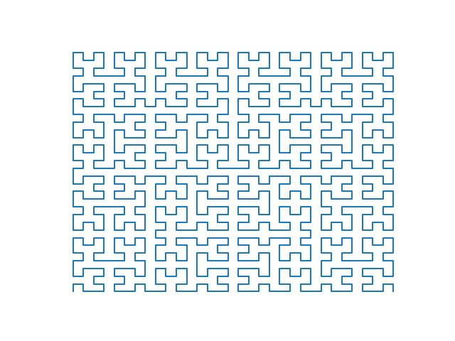
For more detailed explanation of Hilbert curves I recommend you to read chapter 16 in Hacker's Delight 2nd Edition. The method used in this post for calculating positions was taken from the book.
Implementation
From the distance $s$ (number of steps taken) traversed along the grid the current $(x, y)$ coordinates can be determined. For the Ising Model simulation a parallel prefix algorithm was chosen as it is efficient for calculating positions for Hilbert curves with large order numbers. In grid.rs:
use rand::prelude::*;
use std::fs::File;
use std::io::{Error, Write};
#[derive(Debug, Clone)]
pub struct SpinGrid {
    dim_x: usize,
    dim_y: usize,
    order: Option<usize>,
    pub grid: Vec<Vec<i32>>, //2D spin grid
}
impl SpinGrid {
//...
    pub fn new_hcurve(order: usize) -> Self {
        let dim = 1 << order;
        SpinGrid {
            dim_x: dim,
            dim_y: dim,
            order: Some(order),
            grid: vec![vec![1; dim]; dim],
        }
    }
//...
    pub fn calculate_configurations_hcurve(
        &mut self,
        inter_strength: f64,
        temperature: f64,
    ) -> Result<(), &'static str> {
        let mut rng = rand::thread_rng();
        //parallel prefix method is used to get (x, y) from Hilbert curve distance s
        if let Some(n) = self.order {
            let max_length = (1 << n) * (1 << n);
            for i in 0..max_length {
                let mut s = i | (0x55555555 << (2 * n));
                let sr = (s >> 1) & 0x55555555;
                let mut cs = ((s & 0x55555555) + sr) ^ 0x55555555;
                cs = cs ^ (cs >> 2);
                cs = cs ^ (cs >> 4);
                cs = cs ^ (cs >> 8);
                cs = cs ^ (cs >> 16);
                let swap = cs & 0x55555555;
                let comp = (cs >> 1) & 0x55555555;
                let mut t = (s & swap) ^ comp;
                s = s ^ sr ^ t ^ (t << 1);
                s &= (1 << (2 * n)) - 1;
                t = (s ^ (s >> 1)) & 0x22222222;
                s = s ^ t ^ (t << 1);
                t = (s ^ (s >> 2)) & 0x0C0C0C0C;
                s = s ^ t ^ (t << 2);
                t = (s ^ (s >> 4)) & 0x00F000F0;
                s = s ^ t ^ (t << 4);
                t = (s ^ (s >> 8)) & 0x0000FF00;
                s = s ^ t ^ (t << 8);
                let x = s >> 16;
                let y = s & 0xFFFF;
                let sigma_xy = self.grid[x][y] as f64;
                let mut sum = 0;
                if x < self.dim_x - 1 {
                    sum += self.grid[x + 1][y];
                }
                if x > 0 {
                    sum += self.grid[x - 1][y];
                }
                if y < self.dim_y - 1 {
                    sum += self.grid[x][y + 1];
                }
                if y > 0 {
                    sum += self.grid[x][y - 1];
                }
                let s = sum as f64;
                let energy = 2.0 * inter_strength * sigma_xy * s;
                let rn: f64 = rng.gen();
                if energy < 0.0 || rn < (-energy / temperature).exp() {
                    self.grid[x][y] = -self.grid[x][y];
                }
            }
            Ok(())
        } else {
            Err("to calculate configuration with Hilbert curve use SpinGrid::new_hcurve(order) when creating the grid")
        }
    }
/...
}
Let us now compare the computation times and 2D images of spin configurations of the two methods.
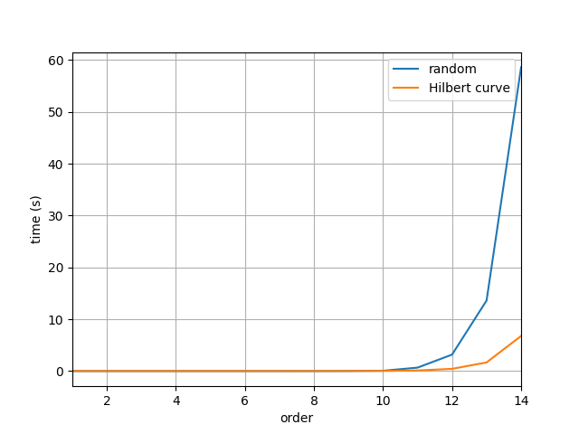
As we can see from the benchmarks above the computation time for the random position method increases significantly more compared to the method that uses Hilbert curve as the grid size increases. The Hilbert curve method is over 10x faster for the $16384\times16384$ grid.
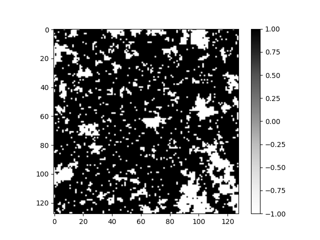
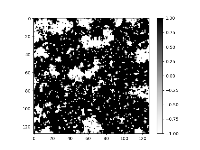
As we can see from the 2D images the configurations resemble each other. There is no signs of the Hilbert curve pattern in the 2D image. This is partly due to the amount of Monte Carlo steps. As the amount of steps increases the influence of randomness provided by the Boltzmann distribution increases and the images start to look alike regardless of the method.
Conclusion
In this post we have managed to speed up our 2D Ising model simulation considerably. The images provided by the Hilbert curve method resemble the ones obtained with the random position method and no traces of the curve pattern were seen on the 2D images.