Using the Metropolis-Hastings algorithm to simulate the 2D Ising model
Introduction
In this post we will be implementing and using the Metropolis-Hastings algorithm to calculate the spin configuration of the 2D Ising model based on a paper written by Jean-Charles Walter and Gerard Barkema in 2014. The algorithm belongs to a group of Markov chain Monte Carlo (MCMC) methods that are used in numerical analysis and to calculate multiple integrals.
2D Ising Model
The Ising model was originaly invented by physicist Wilhelm Lenz in 1920 and given as a problem to his student Ernst Ising. The model describes the configuration of the magnetic dipole moments of atomic spins in a set of lattice sites. Consider a two dimensional grid consisting of lattice sites adjacent to each other with each lattice site $k$ having a spin $\sigma_k=\pm1$. Between a lattice site $i$ and their neighboring site(s) $j$ there exists a interaction $J_{ij}$. In our simulation the external magnetic field is considered to be zero and the neighbor interaction $J$ is the same for all sites. The energy of a configuration $\sigma_{x,y}$ in the 2D grid is given by the Hamiltonian function
\[\mathcal{H}_{xy}=-J\sigma_{x, y}(\sigma_{x-1, y}+\sigma_{x+1, y}+\sigma_{x, y-1}+\sigma_{x, y+1}).\]When the system has reached equilibrium at temperature $T$, the probability of the configuration $\sigma_{x, y}$ is given by the Maxwell-Boltzmann factor
\[P(\sigma_{x, y})=\frac{e^{-\frac{\mathcal{H}_{xy}}{k_BT}}}{Z},\]where $k_B$ is the Boltzmann factor and $Z$ is the partition function.
Metropolis-Hastings method
Ergodicity and the condition of detailed balance
Ergodicity and the condition of detailed balance are important terms when implementing Monte Carlo simulations. During a Monte Carlo simulation a small random change in configuration $C_i$ is proposed to the system resulting in the trial configuration $C^t_{i+1}$. The trial configuration is then either accepted resulting in $C_{i+1}=C^t_{i+1}$ or rejected resulting in $C_{i+1}=C_i$. This set of configurations $i=1, …, M$ is called a Markov chain in the phase space of the system. Markov process can be described by equation
\[\dfrac{d}{dt}P_A(t)=\sum_{A\neq B}\left[P_B(t)W(B\rightarrow A)-P_A(t)W(A\rightarrow B)\right],\]where $P_A(t)$ is the propability of configuration $A$ at time $t$, $W(A\rightarrow B)\geq0$ is the transition rate for the state $A$ to State $B$. For the transition rate $\sum_B W(A\rightarrow B)=1$ for all $A, B$.
Ergodicity is a constraint which states that starting from any configuration $C_0$ with nonzero probability, any other configuration with nonzero probability can be reached through finite number of proposed changes to the configuration (Monte Carlo moves).
The second constraint is the condition of detailed balance
\[P_AW(A\rightarrow B)=P_BW(B\rightarrow A).\]Since our Ising model is at equilibrium and thus $\dfrac{d}{dt}P(\sigma_{x, y})=0$, this constraint is satisfied. From the equation for the condition of detailed balance we get a ratio of probabilities
\[\frac{W(\sigma_{x, y}\rightarrow -\sigma_{x, y})}{W(-\sigma_{x, y}\rightarrow \sigma_{x, y})}=\frac{P(-\sigma_{x, y})}{P(\sigma_{x, y})}=e^{-\frac{2J\sigma_{x, y}(\sigma_{x-1, y}+\sigma_{x+1, y}+\sigma_{x, y-1}+\sigma_{x, y+1})}{k_BT}}=e^{-\frac{\Delta E}{k_BT}}.\]This ratio of probabilities gives us information on the transition probability of the configuration.
Transition and acceptance probabilities
The rate of change is formed using transition and acceptance probabilities
\[W(A\rightarrow B)=T(A\rightarrow B)A(A\rightarrow B).\]In our Ising model containing $N$ spins the transition probability for a single configuration is $\frac{1}{N}$. For the acceptance probability we use the ratio of probabilities introduced earlier. Probabilities can not exceed 1, so the boltzmann factor ($\Delta E<0$) giving a value bigger than 1 is capped in the simulation. In Metropolis-Hastings algorithm, the acceptance probability is defined as
\[A(\sigma_{x, y}\rightarrow-\sigma_{x, y})=\min\left[1, \frac{P(-\sigma_{x, y})}{P(\sigma_{x, y})}\right]=\min\left[1, e^{-\frac{\Delta E}{k_BT}}\right]\]In terms of physics this makes sense given the principle of minimum energy.
Structure of the algorithm
The algorithm for our 2D Ising Model is summarized by the following steps:
- Initialize all spins to $1$ (up)
- Perform $N=L_{x}L_{y}$ trial moves $L_x$ and $L_y$ being the grid width and height respectively:
- Randomly select a site
- Compute the energy difference $\Delta E$.
- Generate a random number $\mathbf{rn}$ uniformly distributed in $[0, 1]$
- if $\Delta E < 0$ or if $\mathbf{rn} < e^{-\frac{\Delta E}{k_BT}}$: flip the spin.
- Analyze the configuration
In grid.rs:
use rand::prelude::*;

#[derive(Debug, Clone)]
pub struct SpinGrid {
    dim_x: usize,
    dim_y: usize,
    pub grid: Vec<Vec<i32>>, //2D spin grid
    inter_strength: f64,     //normalized interaction strength J/k
    temperature: f64,
}

impl SpinGrid {
    pub fn new(dim_x: usize, dim_y: usize, inter_strength: f64, temperature: f64) -> Self {
        SpinGrid {
            dim_x,
            dim_y,
            grid: vec![vec![1; dim_y]; dim_x], //initialize grid with all spins up
            inter_strength,
            temperature,
        }
    }

    pub fn calculate_configurations(&mut self) {
        let mut rng = rand::thread_rng();

        let n = self.dim_x * self.dim_y;
        for _i in 0..n {
            let x: usize = rng.gen_range(0..self.dim_x);
            let y: usize = rng.gen_range(0..self.dim_y);
            let sigma_xy = self.grid[x][y] as f64;
            let mut sum = 0;

            if x < self.dim_x - 1 {
                sum += self.grid[x + 1][y];
            }

            if x > 0 {
                sum += self.grid[x - 1][y];
            }

            if y < self.dim_y - 1 {
                sum += self.grid[x][y + 1];
            }

            if y > 0 {
                sum += self.grid[x][y - 1];
            }

            let s = sum as f64;
            let energy = 2.0 * self.inter_strength * sigma_xy * s;

            let rn: f64 = rng.gen();
            if energy < 0.0 || rn < f64::exp(-energy / self.temperature) {
                self.grid[x][y] = -self.grid[x][y];
            }
        }
    }
}
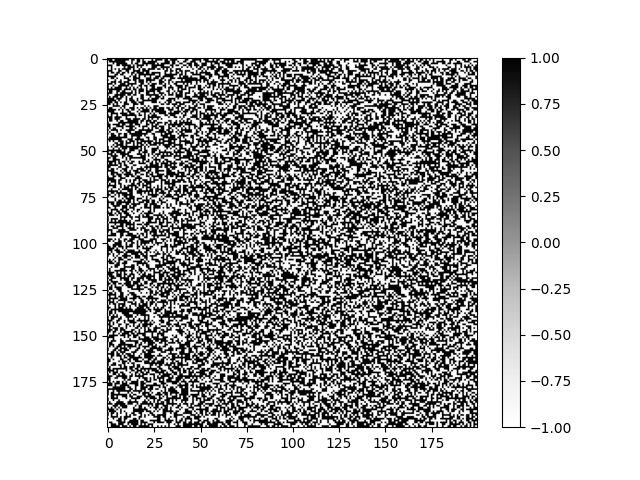
In this implementation interaction strength is normalized with $k_B$. Let us run the algorithm on a $200\times200$ grid with interaction strength $\frac{J}{k_B}=1$ and temperature $T=200$ K (these values may not be accurate in a physical sense). We get the following image:
The End
And that’s a wrap! We have implemented a Metropolis-Hastings algorithm to simulate a 2D Ising model without external magnetic field. If you come accross any flaws in the implementation or in the explanation of the theory please let me know via email. Improvement suggestions for the implementation are also welcome!